

Welcome to the third Wellbore Wednesdays from Madala. In the last couple of weeks we’ve been looking at the performance of extended-reach SAGD wells, starting with tailpipe completions, followed by the realization that tailpipes can really constrain how much you can draw on a long liner, followed by a simpler liner with no tailpipe that has a lot more production capacity. You can get caught up here if you haven’t seen the series yet:
Simulating Performance of Extended-Reach SAGD wells – part 2
This week we’re looking at inflow and what it means for production capacity. When we started out, we were looking at the flow capacity of the completion and made the assumption that inflow along the liner was evenly distributed. That’s fine for looking at hydraulics in general but it’s not really valid. If we’re going to make an assumption about evenly-distributed inflow, it should be an evenly-distributed ability to deliver from the reservoir, as if you had the same permeability and porosity along the liner, which would deliver the same inflow rate with the same pressure gradient everywhere. In reality, the reservoir isn’t going to be uniform, the rock properties change, injection impacts the chamber over the life of the well and so on.
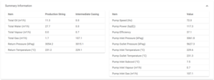
We recalibrated the extended-reach well with a constant Productivity Index (PI) inflow model that delivered the same rates as the even-inflow model. The even-inflow rates are here:
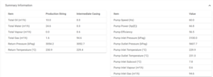
The PI rates are the same except for some negligible differences:
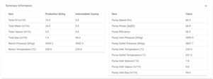
At these rates, the liner had a 30 kPa dP from toe to heel, which is low. We wanted to look at how much more production was available at this PI. The simple lever for this is pump speed. The first step was to increase pump frequency by 10% to 66 Hz:
This is good, we have 8% more production. Another step to 72 Hz:
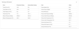
This delivers 13% more over the base. One more step to 75Hz:
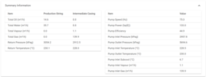
This is a large increase over base, 46% more. If you look at the Pump Inlet Pressure or FBHP for each case, you can see why. The base case is at 3099.5 kPag. It’s 3078 at 66 Hz and it’s 3062 at 72 Hz. At 75 Hz though it’s 2958 kPag. The liner pressure is a lot lower and increases the draw on the reservoir. The pressure profile for this case is below:
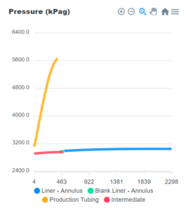
The liner itself still doesn’t have a large toe-heel pressure drop, it’s still only 50 kPa compared to the base case of 30 kPa. The liner isn’t limiting at all, compared to what we saw with the shorter liners that had tailpipes. It might be possible to deliver these rates with a smaller-diameter liner, which is cheaper. Alternatively, there may be more production potential. ICDs may be able to help with delivering higher rates. This is where inflow needs to be analysed with the reservoir team and fed back into the design to maximise performance vs cost. The oil rate in field units is around 2200 bbl/d for this case. At a $60/bbl bitumen netback, the well makes $132,000 a day, so it’s worth getting the design right to see what’s achievable.
As a final note, we know the ESP in this case is wrong for this design. You wouldn’t design for 75 Hz. Frequency was just the lever for testing the inflow deliverability. Pump wear is proportional to the cube of frequency, so at 75 Hz you would cut the lifetime of the pump in half, let alone the impact of the extra heat.
Next week we’ll look at the impact of different PI distributions along the liner and the potential for ICDs. Please reach out to Raj Bal, Stan Cena or Damien Hocking if you’d like to learn more, and follow us to keep up on the Wellbore Wednesdays series.